Statistics for Data Science: Confidence Intervals

Confidence Intervals. Image Source: https://nulib.github.io/moderndive_book/10-CIs.html

A population is defined by parameters such as mean and variance and standard deviation. But finding these values for a population can be difficult or impossible because it is not usually easy to collect data for every single subject in a large population.

So instead of collecting data in the entire population, we choose a subset of the population and call it a sample. We calculate the mean and standard deviation for the sample and use these as point estimates for our population distribution.

But the problem with these point estimates is that we don't know how good our point estimates are. Depending upon the sampling points and sample size, the point estimates might be a great estimate of the population parameter, or they might be a really bad estimate. So it might be really helpful to be able to say how confident we are about how well the sample estimates are estimating the population parameter. That’s where the confidence intervals come into the picture.

So while the point estimates are easy to calculate, the drawback is that they don't tell us how bad or good the estimate really is. In contrast, we have interval estimates, which give us a range of estimates in which the point estimate may lie. It's a little harder to calculate than a point estimate, but it gives us much more information.

With interval estimates, we are able to make statements like “I’m 95% confident that the population mean lies in the interval (a,b),” or “I’m 99% confident that the population proportion lies in the interval (a,b).”

These 95% and 99% values that we are referring to are called confidence intervals. A confidence interval is a probability that an interval estimate will include the population parameter. We usually choose a 90%, 95% or 99% as the confidence level, and then find the interval associated with that confidence level.

Alpha and the region of rejection

Corresponding to every confidence interval that we choose( for example 95%) above, there is a region 𝛼(5%) that won’t contain the population parameter. This 5% region is called the alpha value or the level of significance or the probability of making a Type I error. So 𝛼 = 1- confidence level.

We can visualise 𝛼 as the total area under the normal distribution outside of the confidence interval. For example, given a 90% confidence level, the alpha value is

𝛼 = 1–0.90

𝛼 = 0.10

Confidence Interval and 𝛼 values. Source: https://saylordotorg.github.io/text_introductory-statistics/s11-01-large-sample-estimation-of-a-p.html

Since the confidence interval is always centred around the mean of the normal distribution, we can show that the central 1-𝛼, and half of 𝛼 in the lower tail to the left of the confidence interval, and the other half of 𝛼 in the upper tail to the right of the confidence interval.

In other words, at a 90% confidence interval, we can expect the smallest 5% and largest 5% of values to fall outside the confidence interval, because 𝛼 is evenly split into the lower and upper tails.

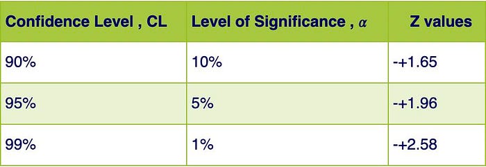
Using a z-table, we can find that the values associated with -0.05 and 0.05 are -1.65 and 1.65 respectively, which means the boundaries of the 90% confidence interval are -1.65 and 1.65.

From this, we can conclude that any z-value outside of z = ±1.65 will put us outside the 90% confidence interval, and inside the region of rejection. So these z values are the boundaries of the region of rejection, for a 90% confidence level.

We can use this chart for the most common values of the confidence levels, and the corresponding level of significance and z-values.

Image By Author

Confidence Interval when 𝛔 is known

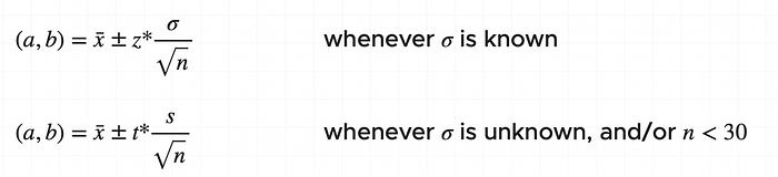
When population standard deviation is known, the confidence interval (a,b) is given by

(a,b) = ẍ ± 𝒛* (𝛔/√n)

where

(a,b) is the confidence interval,

ẍ is the sample mean,

𝒛* is the z-score for the confidence-level chosen,

𝛔 is the population standard deviation, and

n is the sample size

The term 𝒛* (𝛔/√n) is also known as the margin of error, so the confidence interval can also be given by

(a, b) = ẍ ± margin of error

From the formula above, it can be said that,

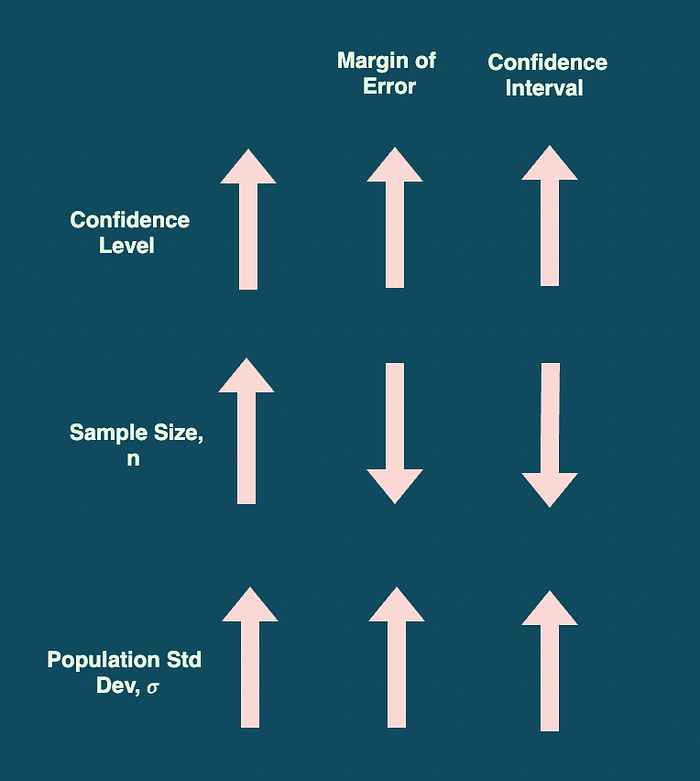
• The higher the confidence level, the wider the confidence interval (because as z* gets larger, the margin of error term becomes larger, which makes the entire confidence interval wider).
• The larger the population standard deviation 𝜎, the more the margin of error, the wider the confidence interval.
• The larger the sample size n, the narrower the confidence interval (because as n gets larger, the margin of error will become smaller, making the confidence interval narrower).

Image by Author

In general, we want the smallest confidence interval we can get, because the smaller the confidence interval, the more accurately we can estimate the population parameter.

Confidence Interval when population standard deviation 𝛔, is unknown and/or we have a small sample

In cases when 𝛔 is unknown, we use t-value, from the student’s t -distribution, instead of z-value from the normal distribution to find the confidence interval.

(a, b) = ẍ ± t* (s/√n)

where s is the sample standard deviation and t* is the t-value for the confidence level chosen.

Similarly, if the sample size is small (n < 30), then we don’t have enough data for the Central Limit Theorem to reliably apply, and we use t-value in this case too.

So our confidence interval formula can be given by

Sample size for fixed margin of error

Often we want to find the smallest possible sample size, in order to stick to a specific margin of error. Since the margin of error is given by,

ME = z*σ/√n

we can find the sample size n, for a given confidence level and ME by using

n = (z*𝜎/ME)²

Related Articles:

Statistics for Data Science : P-value in Hypothesis Testing

Statistics for Data Science: Central Limit Theorem

Statistics for Data Science: Visualising Conditional Probability

Statistics for Data Science: Normal Distribution, Z-score and Chebyshev’s Theorem

Thanks for reading. Your comments, feedback and suggestions are welcome.